Part 1. Systems
1.2.1 自变量变换举例
Time reflection 时间反转: x(t)⟷x(−t), x[n]⟷x[−n]
Time scaling 时间尺度变换: x(t)⟷x(ct)
Time shift 时移: x(t)⟷x(t−t0), x[n]⟷x[n−n0]
To perform transformation x(t)→x(αt+β), you have to do time-shifting and then scaling 先时移再时间尺度变换.
E.g. x(t)→x(t+β)→x(αt+β)
1.2.3 Even and odd signal 偶信号与奇信号
Ev{x(t)}=21(x(t)+x(−t))
Od{x(t)}=21(x(t)−x(−t))
1.3 Exponential and sinusoidal Signal 指数信号与正弦信号
Euler’s formula: ejωt=cos(ω0t)+j⋅sin(ω0t)
Sinusoidal signal: x(t)=Acos(ω0t+ϕ)
Sinusoidal signal can be written in terms of periodic complex exponentials with the same fundamental frequency:
Acos(ω0t+ϕ)=2Aejϕejω0t+2Ae−jϕe−jω0t
1.3.1 连续时间复指数信号与正弦信号
- x(t)=ejω0t
- T0=2π/∣ω0∣
1.3.2 离散时间复指数信号与正弦信号
1.4 Unit Impulse and Unit Step function
1.4.1 DT Unit impulse & Unit step
Unit impulse function δ[n] and u[n]
δ[n]={0,1,n=0n=0, u[n]={0,1,n<0n≥0
δ[n]=u[n]−u[n−1]
1.4.2 CT Unit impulse & Unit step
- Unit impulse function δ(t) and u(t)
u(t)={0,1,n<0n>0, δ(t)=dtdu(t)
1.6 Properties of System 基本系统性质
1. Memoryless: output only depends on input at the same time 当前输出仅依赖当前输入
2. Invertibility: distinct inputs lead to distinct outputs 不同输入导致不同输出,输入和输出一一对应
3. Causality: output doesn’t depend on future 不依赖未来的输入,仅依赖过去和现在的输入
现实中的系统都是因果系统
All memoryless are casual ! 无记忆系统都是因果系统
4. Stability: bounded input gives bounded output 输入有界则输出有界
5. Time-invariance: a time shift in the input only causes a time shift in the output
If x[n]→y[n], then x[n−n0]→y[n−n0]
6. Linearity: a system is linear if (1)additivity and (2)scaling
Part 2: LTI system
2.1 DT LTI System 离散时间线性时不变系统:卷积和
x[n]=k=−∞∑∞x[k]δ[n−k]
- 对于任意LTI,只需知道输入信号和单位冲激响应,求卷积和,就能得到输出
y[n]=x[n]∗h[n]=k=−∞∑∞x[k]h[n−k]
2.2 CT LTI System 连续时间线性时不变系统:卷积积分
x(t)=∫−∞∞x(τ)δ(t−τ)dτ
y(t)=x(τ)∗h(τ)=∫−∞∞x(τ)h(t−τ)dτ
2.3 LTI system properties 线性时不变系统的性质
Commutative 交换律: x(t)∗h(t)=h(t)∗x(t) (离散同理)
Bi-linear? 分配律: (ax1(t)+bx2(t))∗h(t)=a(x1∗h)+b(x2∗h), x∗(ah1+bh2)=a(x∗h1)+b(x∗h2)
Shift: x(t−τ)∗h(t)=x(t)∗h(t−τ) ( 例如x(t−2)∗h(t+2)=x(t)∗h(t) )
Identity: δ(t) is the identity signal, x∗δ=x=δ∗x
Associative: x1∗(x2∗x3)=(x1∗x2)∗x3
2.3.4 Memoryless LTI systems
- h[n]=0 for n=0
2.3.5 Invertibility of LTI systems
A system is invertible only if an inverse system exists
h(t)∗h1(t)=δ(t)
2.3.6 Casuality of LTI systems
- h[n]=0 for n<0
2.3.7 Stability of LTI systems
- If ∑k=−∞∞∣h[k]∣<∞ (绝对可和) / ∫−∞∞∣h(τ)∣dτ<∞, then y[n] is bounded, and the system is stable.
δ(t)∗δ(t)=δ(t)
Derivatives
y′(t)=x′(t)∗h(t)=x(t)∗h′(t)
y(k+r)(t)=x(k)(t)∗h(r)(t)
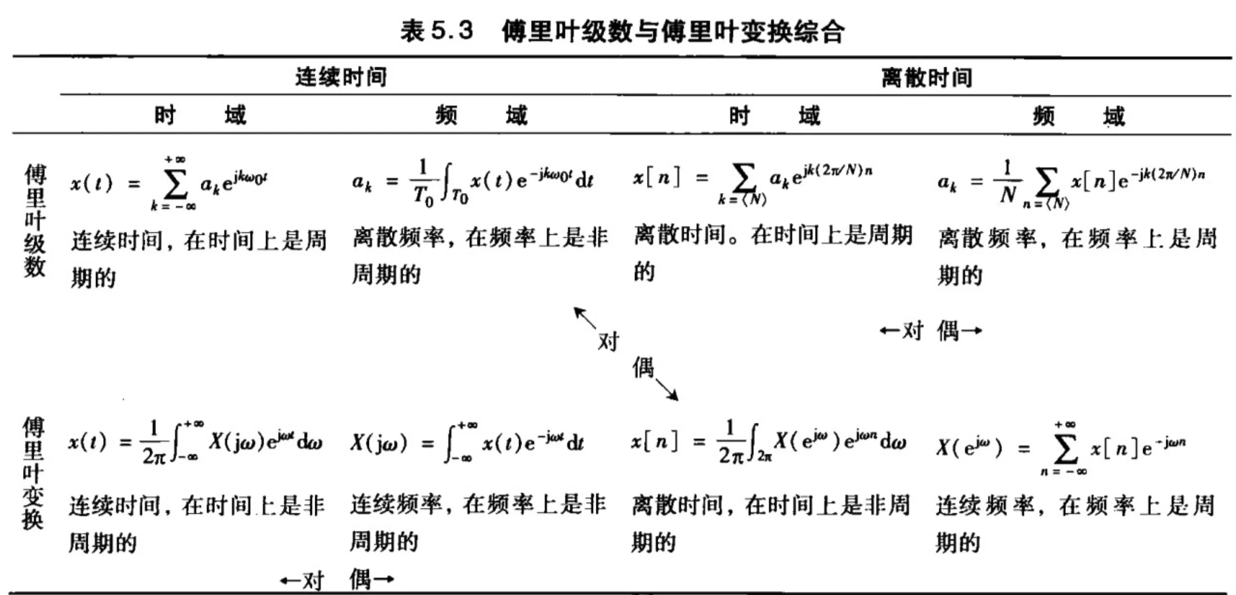
Part 3: Fourier series
Euler’s Formula
ejx=cos(x)+jsin(x)
sin(x)=2jejx−e−jx
cos(x)=2ejx+e−jx
3.2 Eigenfunction of LTI system
(线性时不变系统对复指数信号的响应)
如果有一个函数进入系统后,系统的输出是函数的常数倍(可能是复数),那么这个函数就是这个系统的特征函数 eigenfunction
CT
x(t)=est→y(t)=est∫−∞∞h(τ)e−sτdτ=est⋅H(s)
- Eigenfunction: est
- Eigenvalue: H(s)=∫−∞∞h(τ)e−sτdτ
DT
x[n]=zn→y[n]=znk=−∞∑∞h[k]z−k=zn⋅H(z)
- Eigenfunction: zn
- Eigenvalue: H(z)=∑k=−∞∞h[k]z−k
Usefulness
如果 x(t) 能写成一堆eigenfunction的加权之和,那么我们就能很容易知道 x(t) 的输出。
CT: DT: x(t)=k∑akesktx[n]=k∑akzkn⇒y(t)=k∑akH(sk)eskt⇒y[n]=k∑akH(zk)zkn
Fourier Analysis
For fourier analysis, we consider:
CT: pure imaginary exponential: est=ejωt
Input: ejωt, Output: H(jω)ejωt
DT: Unit: zn=ejωn
Input: ejωn, Output: H(ejω)ejωn.
3.3 连续时间周期信号的Fourier级数表示
3.3.1 An orthonormal set 成谐波关系的复指数信号的线性组合
S={x(t)∣x(t)=x(t+T0),∀n}, T0=ω02π
Dot product (Inner product): <x1(t),x2(t)>=T1∫−2T2Tx1(t)x2∗(t)
Harmonically related complex exponential: B={ϕk(t)∣ϕk(t)=ejkω0t,k∈Z}
Observe that they are orthonormal:
2πω0∫−ω0πω0πejk1ω0te−jk2ω0t=δ[k1−k2]={01k1=k2k1=k2
3.3.2 Fourier Series Expansion 连续时间周期信号傅里叶级数表示的确定
Theorem: x(t) may be expressed as a Fourier series and ak can be obtained by
x(t)=k=−∞∑∞akejkω0t, ak=T01∫T0x(τ)e−jkω0τdτ
a0 可以直接用面积除以周期计算:
a0=T01∫T0x(τ)dτ
方波的Fourier Series
a0=T2T1,ak=kπsin(kω0T1)
Decomposition of Even and Odd
In general, ak is complex, therefore this is not real and imaginary decomposition. However, this is the even and odd decomposition.
不是实部和虚部的分解,而是偶函数与奇函数的分解。
x(t)=k=−∞∑∞akejkω0t=k=−∞∑∞(akcos(kω0t)+jaksin(kω0t))=a0+k>0∑((ak+a−k)cos(kω0t)+j(ak−a−k)sin(kω0t))
x(t) even → all sine terms vanish → ak=a−k
x(t) odd → all cosine terms vanish → ak=−a−k
3.5 Properties of CT Fourier Series 连续时间傅里叶级数的性质
x(t)⟷FSak
Linearity: z(t)=αx(t)+βy(t)⟷FSαak+βbk
Time-shift: x(t−t0)⟷FSe−jkω0t0ak
Time-Reverse: x(−t)⟷FSa−k
Time-scaling: x(αt)=∑k=−∞∞akejk(αω0t)
Multiplication: x(t)y(t)⟷FShk=∑l=−∞∞albk−l
Conjugation & conjugate Symmetry : x∗⟷FSa−k∗
If x(t) is real, then x(t)=x∗(t), ak∗=a−k
If x(t) is real and even, ak=a−k=ak∗, FS coefficients are real and even.
If x(t) is real and odd, ak=−a−k=−ak∗, FS coefficients are purely imaginary and odd.
Derivative and integral: dtdx(t)⟷FSjkω0ak, ∫−∞tx(τ)dτ⟷FSjkω0ak
Parseval’s Identity: T1∫T∣x(t)∣2=∑k=−∞∞∣ak∣2
3.6 Fourier series for DT Periodic signal 离散时间周期信号的傅里叶级数表示
与连续时间周期信号的区别:有限项级数;不存在收敛问题
3.6.1 An orthonormal set 成谐波关系的复指数信号的线性组合
- The set T of x[n] satisfying x[n]=x[n+N]
- Dot product (inner-product) defined as
<x1[n],x2[n]> =N1n=0∑N−1x1[n]x2∗[n]
- The set C of N functions in T
μk[n]=ejkω0n;0≤k≤N−1
- Observe that they are orthonormal:
N1m=0∑N−1ejkω0me−jk2ω0m={0,k1=k21,k1=k2
3.6.2 Fourier Series for DT Periodic signal
Theorem:
x[n]=k=0∑N−1akejkω0n,ak=N1m=0∑N−1x[m]e−jkω0m
3.7 Properties of DT Fourier Series 离散时间傅里叶级数性质
x(t)⟷FSak
- Linearity: Ax[n]+By[n]⟷FSAak+Bbk
- Time-shift: x[n−n0]⟷FSake−jkω0n0
- Frequency Shifting: ejMω0nx[n]⟷FSak−M
- Conjugation: x∗[n]⟷FSa−k∗
- Time reversal: x[−n]⟷FSa−k
- Periodic convolution: ∑r=<N>x[r]y[n−r]⟷FSNakbk
- Multiplication: x[n]y[n]⟷FS∑l=<N>albk−l
- First difference: x[n]−x[n−1]⟷FS(1−e−jkω0)ak
- Parseval’s relation: N1∑n=<N>∣x[n]∣2=∑k=<N>∣ak∣2
3.8 Fourier Series and LTI system 傅里叶级数与线性时不变系统
CT
System function 系统函数
(Recall) Eigenfunction: x(t)=est→y(t)=H(s)est
where H(s)=∫−∞∞h(τ)e−sτdτ is called system function
Frequency response 频率响应
Consider the special case when Re{s}=0
s=jω→est=ejωt→
H(jω)=∫−∞∞h(t)e−jωtdt
is called frequency response
Output
x(t)=k=−∞∑∞akejkω0ty(t)=k=−∞∑∞akH(jkω0)ejkω0t
Part 4. CTFT 连续时间傅里叶变换
4.1 非周期信号的傅里叶变换
Fourier transform pair
- Inverse Fourier Transform
x(t)=2π1∫−∞∞X(jω)ejωtdω
Fourier transform / Spectrum density function 频谱密度函数
X(jω)=∫−∞∞x(t)e−jωtdt
频谱密度函数一般是复数,所以一般用模长和相位两部分来表示
Duality property of Fourier Transform 对偶性质
F{F{x(t)}}=2πx(−t)
δ(t)⟷FT1
时间域越宽,频域越窄
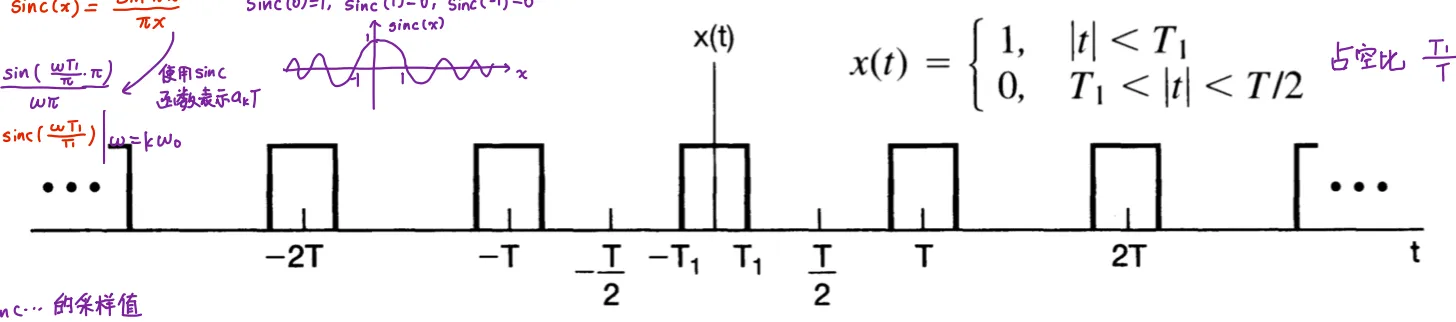
方波的Fourier Transform
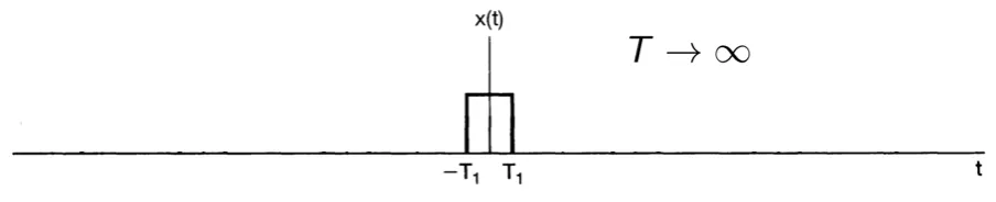
定义sinc(x)=πxsin(πx)
X(jω)=ω2sin(ωT1)=2T1sinc(πωT1)
x(t)⟷FSak ⇒ X(jω)=k=−∞∑∞2π⋅ak⋅δ(ω−kω0)
Notation:
X(jω)=F{x(t)} or x(t)⟷FTX(jω)
Linearity: ax(t)+by(t)⟷FTaX(jω)+bY(jω)
Time-shift: x(t−t0)⟷FTe−jωt0X(jω)
Conjugation: x∗(t)⟷FTX∗(−jω)
Conjugation symmetry: if x(t) is real, X(−jω)=X∗(jω)
If x(t) is real and even, X(jω) is also real and even.
If x(t) is real and odd, X(jω) is purely imaginary and odd.
Differentiation & Integration:
dtdx(t)⟷FTjωX(jω)
∫−∞tx(τ)dτ⟷FTjω1X(jω)+πX(0)δ(ω)
Time and Frequency Scaling:
x(at)⟷FT∣a∣1X(ajω)
x(−t)⟷FTX(−jω)
Duality: F{F{x(t)}}=2πx(−t)
Parseval’s Relation: ∫−∞∞∣x(t)∣2dt=2π1∫−∞∞∣X(jω)∣2dω
4.4 Convolution Property 卷积性质
y(t)=x(t)∗h(t)⟷FTY(jω)=H(jω)⋅X(jω)
4.5 Multiplication 相乘性质
Multiplication in time ⟷FT Convolution in frequency
时间域上的相乘,等于频域上的卷积
r(t)=s(t)p(t)⟷FTR(jω)=2π1[S(jω)∗P(jω)]
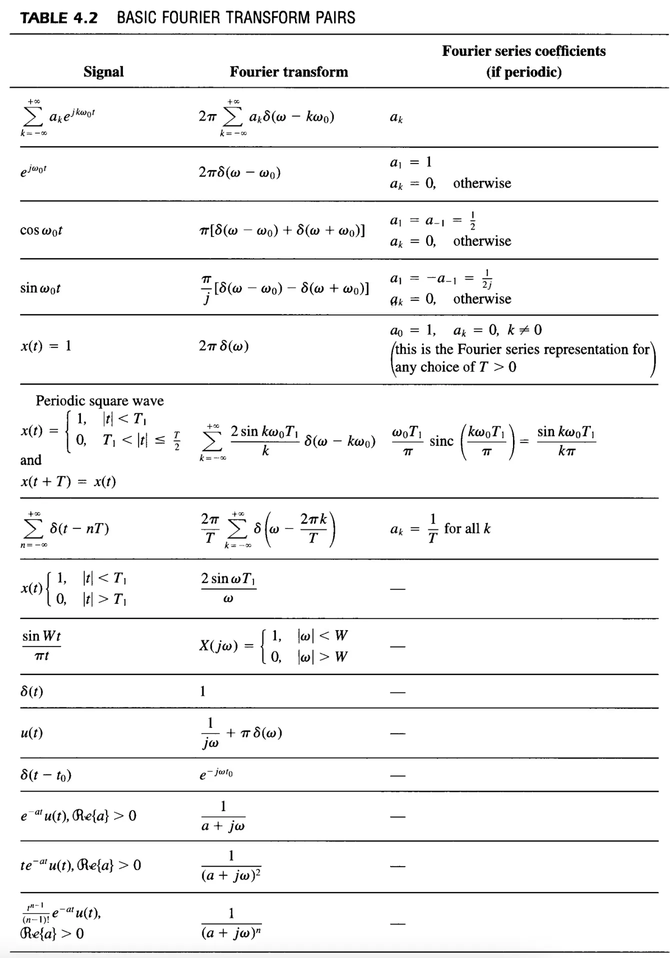
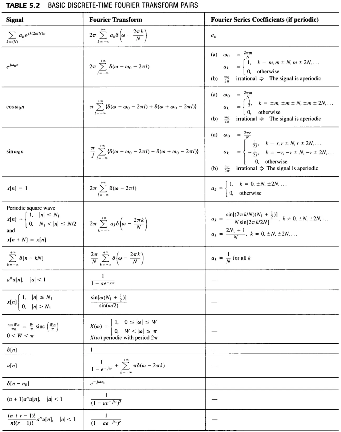
4.6 CTFT pairs
Part 5. DTFT 离散时间傅里叶变换
DTFT
X(ejω)=n=−∞∑∞x[n]e−jωn
X(ejω) is periodic with period 2π.
Inverse DTFT
x[n]=2π1∫−ππX(ejω)ejωndω
Convergence Issues of DTFT 收敛性条件
- x[n] is absolutely summable 绝对可和: ∑−∞∞∣x[n]∣<∞
- OR x[n] has finite energy 有限能量: ∑−∞∞∣x[n]∣2<∞
5.2 DTFT for periodic signals
x[n]⟷FSak ⇒ X(ejω)=−∞∑∞2πakδ(ω−N2πk)
5.3 Properties of DTFT
Notation:
x[n]⟷FTX(ejω)
Periodicity: DTFT is always periodic in ω with period 2π, X(ej(ω+2π))=X(ejω)
Linearity: ax1[n]+bx2[n]⟷FTaX1(ejω)+bX2(ejω)
Time shifting: x[n−n0]⟷FTe−jωn0X(ejω)
Frequency shifting: ejω0nx[n]⟷FTX(ej(ω−ω0))
Conjugation and conjugate symmetry: X∗[n]⟷FTX∗(e−jω)
If x[n] is real, then X(ejω)=X∗(e−jω)
Differencing: x[n]−x[n−1]⟷FT(1−e−jω)X(ejω)
Accumulation: y[n]=∑m=−∞nx[m],
m=−∞∑nx[m]⟷FT1−e−jω1X(ejω)+πX(ej0)k=−∞∑∞δ(ω−2πk)
Time reversal: x[−n]⟷FTX(e−jω)
Differentiation in frequency: nx[n]⟷FTjdωdX(ejω)
Parseval: ∑n=−∞∞∣x[n]∣2=2π1∫2π∣X(ejω)∣2dω
Time expansion: x(k)[n]⟷FTX(ejkω)
5.4 Convolution Property
y[n]=x[n]∗h[n]⟷FTY(ejω)=X(ejω)H(ejω)
5.5 Multiplication Property
y[n]=x[n]⋅h[n]⟷FTY(ejv)=2π1∫−ππX(ejω)H(ej(v−ω))dω
5.7 Duality 对偶性
5.6 DTFT pairs
Part 6 Time & Freq characterization of signals and systems
TODO…
Part 7. Sampling
7.1 用信号样本表示连续时间信号:采样定理
7.1.1 Impulse-Train Sampling 冲激串采样
- Sampling function: p(t)=∑n=−∞∞δ(t−nT)
- Sampling period: T
- Sampling frequency: T2π
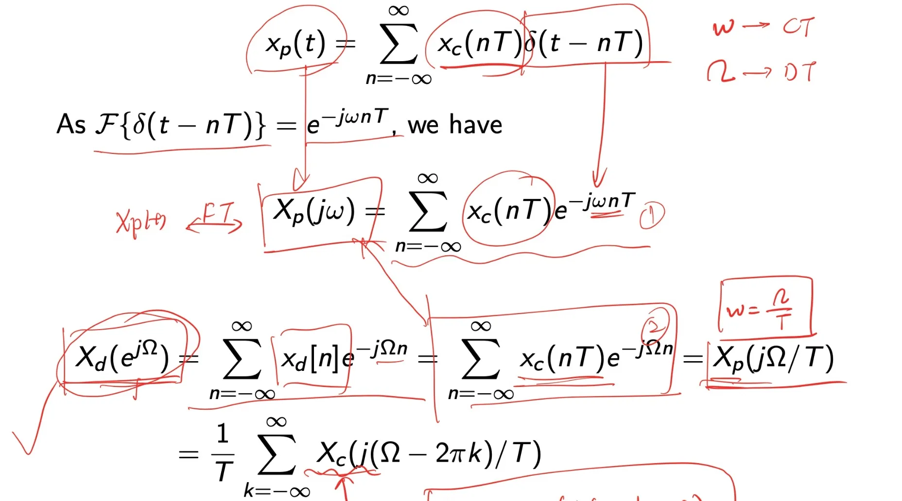
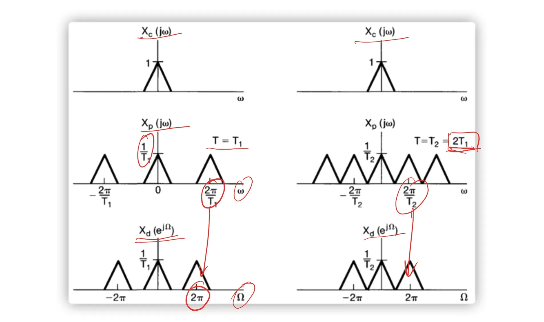
xp(t)=x(t)p(t)=n=−∞∑∞x(nT)δ(t−nT)
Xp(jω)=2π1[X(jω)∗P(jω)]=T1k=−∞∑∞X(j(ω−kωs))
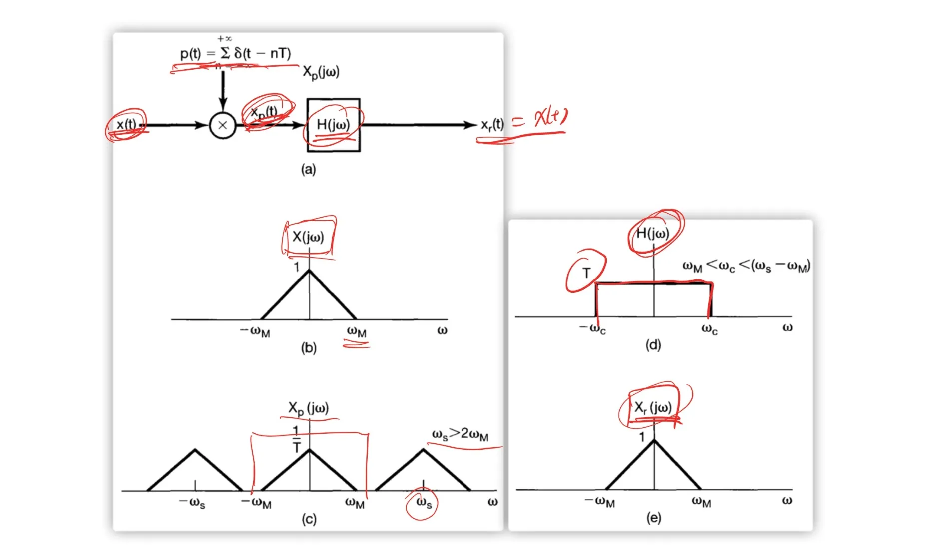
Sampling Theorem:
Let x(t) be a band-limited signal with X(jω)=0 for ∣ω∣>ωM. Then x(t) is uniquely determined by its samples x(nT) if ωs>2ωM, where ωs=T2π
Nyquist rate 奈奎斯特率: 2ωM
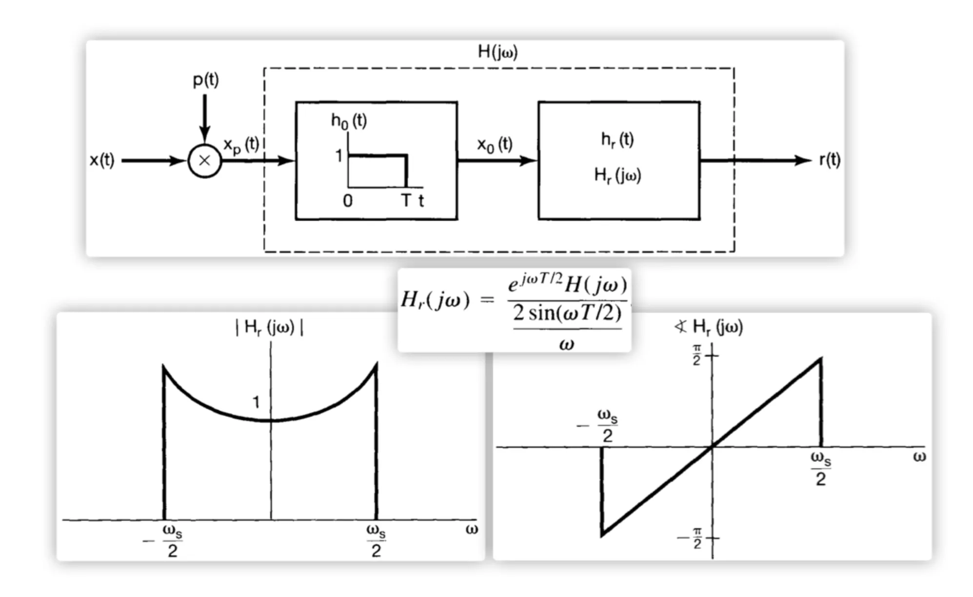
7.1.2 Zero-order Hold Sampling 零阶保持采样
7.2 Signal reconstruction using Interpolation 利用内插重建信号
To be continued…
7.3 Effect of Undersampling: Aliasing 混叠
7.4 Discrete-Time Processing of Continous-Time Signals
Eigenfunction est: H(s)=∫−∞∞h(τ)e−sτdτ
Laplace Transform (LT) of x(t): complex s=σ+jω
x(t)⟷LX(s)=∫−∞∞x(t)e−stdt
X(s)=FT{x(t)e−σt}
X(s)∣s=jω=FT{x(t)}
8.2 Region of Convergence (ROC)
Region of (conditional) convergence 条件收敛: region of s for which
∫−∞∞x(t)e−stdt converges.
Region of (absolute) convergence 绝对收敛: region of s for which
∫−∞∞∣x(t)e−st∣dt converges.
通常使用绝对收敛域
Properties of ROC
ROC consists of strips parallel to the jω-axis.
ROC of rational X(s) does not contain any pole.
If x(t) is of finite duration and absolutely integrable, then ROC is the entire s-plane.
If x(t) is right-sided, and if a line Re(s)=σ0 is in ROC, then ROC contains all s such that Re(s)≥σ0.
If x(t) is left-sided, and if a line Re(s)=σ0 is in ROC, then ROC contains all s such that Re(s)≤σ0.
If x(t) is two-sided, ROC is a strip (can be empty).
Rational X(s), ROC is bounded by poles or extends to infinity.
(1). If x(t) right-sided and X(s) rational, then ROC is the region to the right of the rightmost pole
(2). If x(t) left-sided and X(s) rational, then ROC is the region to the left of the leftmost pole
(3). If x(t) two-sided and X(s) rational, then ROC is a strip between two consecutive poles.
8.3 Inverse LT
x(t)=2πj1∫σ−j∞σ+j∞X(s)estds
8.5 Properties of LT
| Property | Signal | LT | ROC |
|---|
| Linearity | ax1(t)+bx2(t) | aX1(s)+bX2(s) | at least R1∩R2 |
| Time-shift | x(t−t0) | e−st0X(s) | R |
| Shift in s | es0tx(t) | $X(s-s_0) $ | R+Re(s0) |
| Time scaling | x(at) | ∣a∣1X(as) | aR |
| Time reversal | x(−t) | X(−s) | −R |
| Conjugation | x∗(t) | X∗(s∗) | R |
| Convolution | x1(t)∗x2(t) | X1(s)X2(s) | at least R1∩R2 |
| Differentiation in t | dtdx(t) | sX(s) | at least R |
| Differentiation in s | −tx(t) | dsdX(s) | R |
| Integration in t | ∫−∞tx(τ)dτ | s1X(s) | at least R∩{Re(s)>0} |
If x(t)<0 for t<0 and x(t)在t=0不包括任何冲激或高阶奇异函数,
Initial-value theorem: x(0+)=lims→∞sX(s)
Final-value theorem: limt→∞x(t)=lims→0X(s)
Unilateral LT
ROC for a unilateral LT must be a right-half plane, hence ROC is usually omitted.
ULT{x(t)}=LT{x(t)u(t)}
Properties of Unilateral LT
dtdx(t)⟷LsX(s)−x(0−)
dtndnx(t)⟷LsnX(s)−r=0∑n−1sn−r−1x(r)(0−)
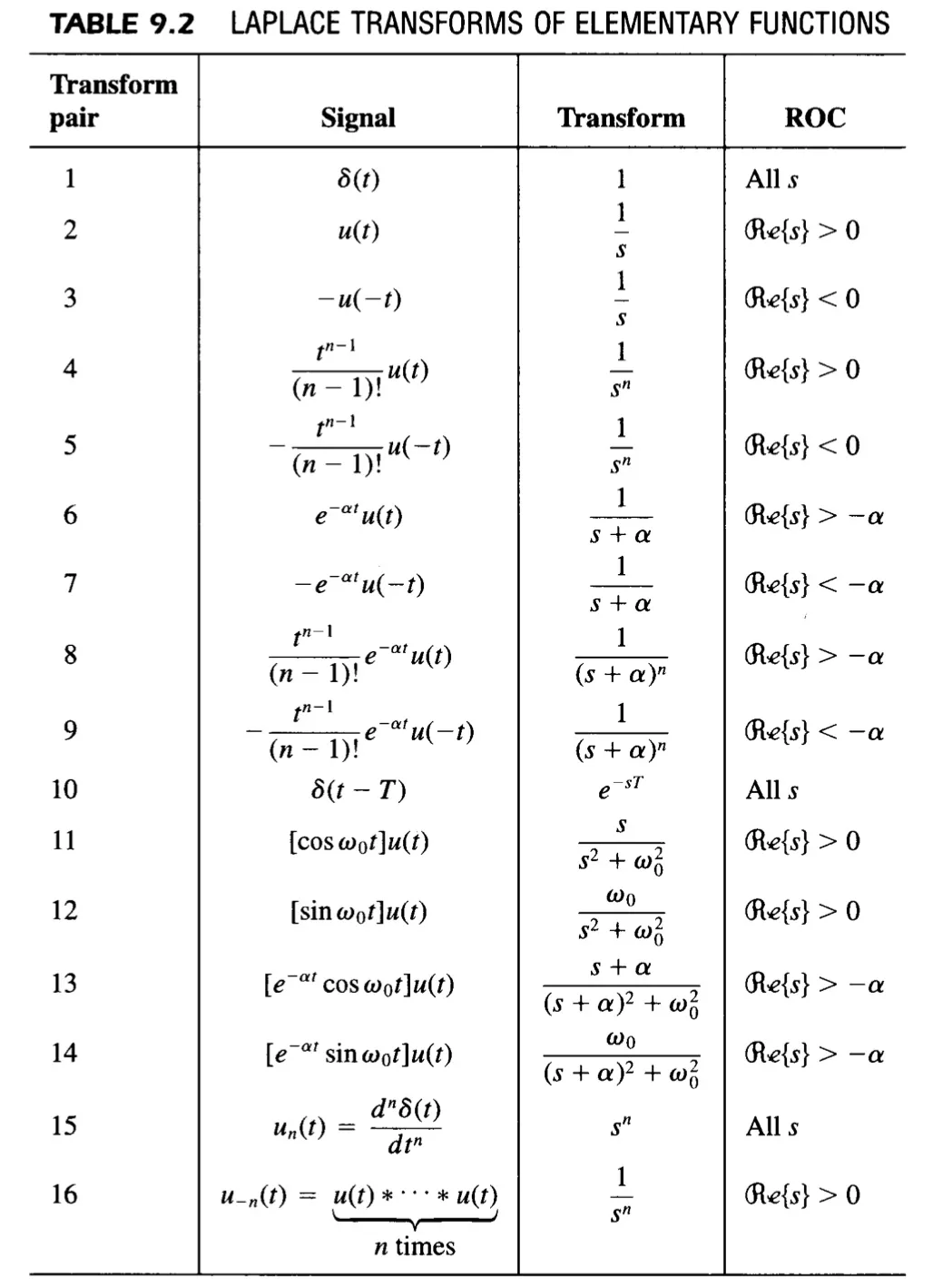
8.6 Some LT pairs
8.7 LTI system and system function
8.7.1 Casuality
For an LTI system, y(t)=x(t)∗h(t), Y(s)=X(s)⋅H(s)
LTI system with H(s): Casual ⇒ ROC is a right-half plane.
LTI system with rational H(s): Casual ⇔ ROC to the right of the rightmost pole
8.7.2 Stability
LTI system with H(s): Stable ⇔ ROC includes jω-axis
LTI system with rational H(s): Casual and stable if and only if all poles lie in the left-half of the s-plane.
8.7.3 LTI system characterized by LCC differential Eqn
To be continued.
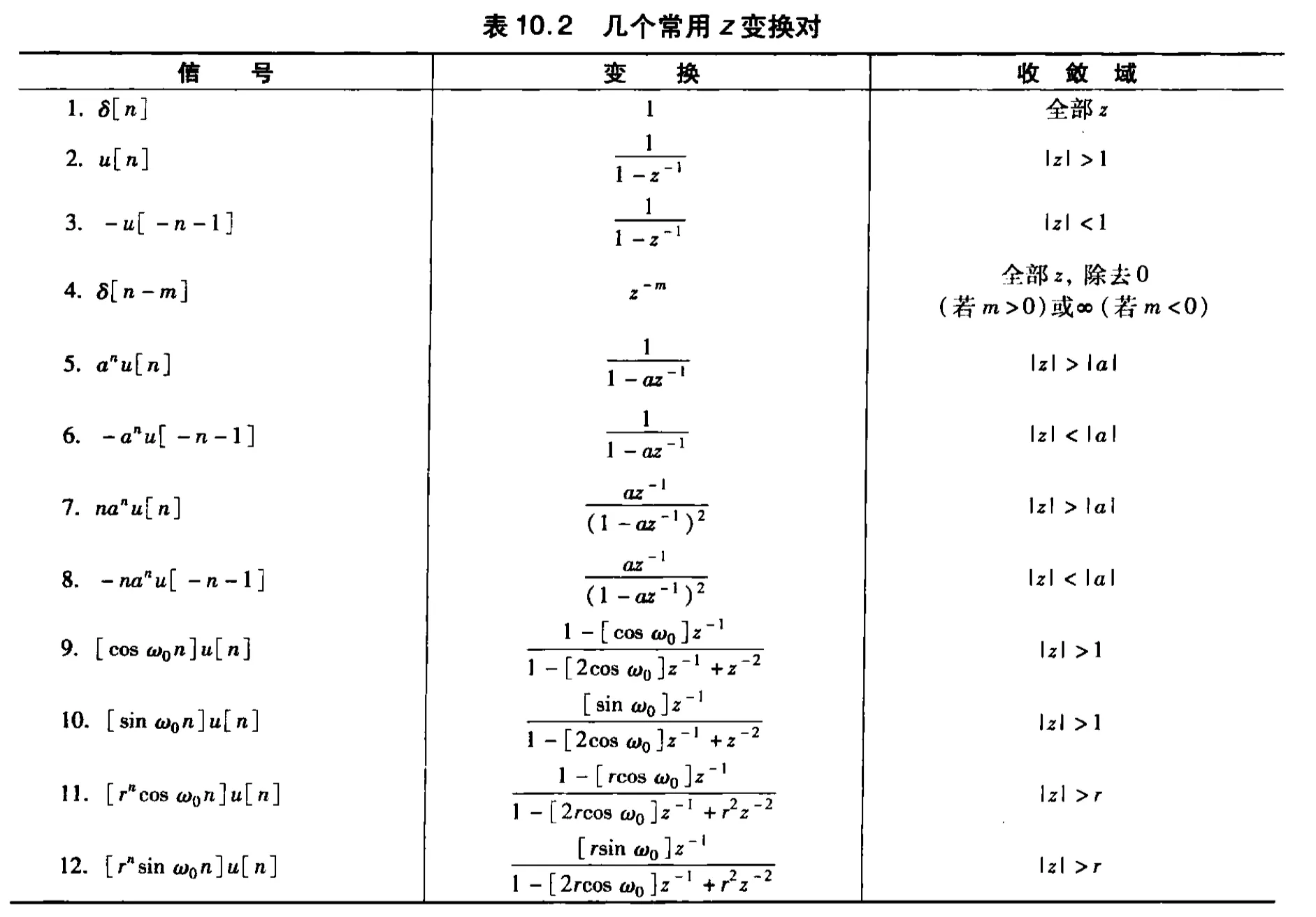
Z
X(z)=n=−∞∑∞x[n]z−n
X(z)=FT{x[n]r−n}
X(z)∣z=ejω=FT{x[n]}
ROC: The set of z such that ∑n=−∞∞∣x[n]zn∣ converges
Properties of ROC
ROC is a ring in the z-plane centered about origin
ROC does not contain any pole.
If x[n] has finite duration, then ROC is the entire z-plane, except possibly z=0 and/or z=∞
(1) If x[n] is right-sided, and if ∣z∣=r0 is in ROC, then all finite values ∣z∣≥r0 will also be in the ROC.
(2) If x[n] is right-sided, then ROC takes the form c<∣z∣<∞.
(1)If x[n] is left-sided, and if ∣z∣=r0 is in ROC, then all finite values ∣z∣≤r0 will also be in the ROC.
(2) If x[n] is left-sided, then ROC takes the form 0<∣z∣<c.
(1) If x[n] is two-sided, and if ∣z∣=r0 is in ROC, then ROC is a ring that includes ∣z∣=r0.
(2) If x[n] is two-sided, then ROC takes the form c1<∣z∣<c2.
If X(z) is rational, then ROC is bounded by poles or extends to infinity.
(1) If x[n] is right-sided and X(z) is rational, then ROC is outside the outermost finite pole (may not include z=∞).
Especially, if x[n] is casual, then ROC contains z=∞
(2) If x[n] is left-sided and X(z) is rational, then ROC is inside the innermost nonzero pole (may not include z=0).
Especially, if x[n] is anticasual, then ROC contains z=0
(3) If x[n] is two-sided and X(z) is rational, then ROC is a ring between two consecutive poles.
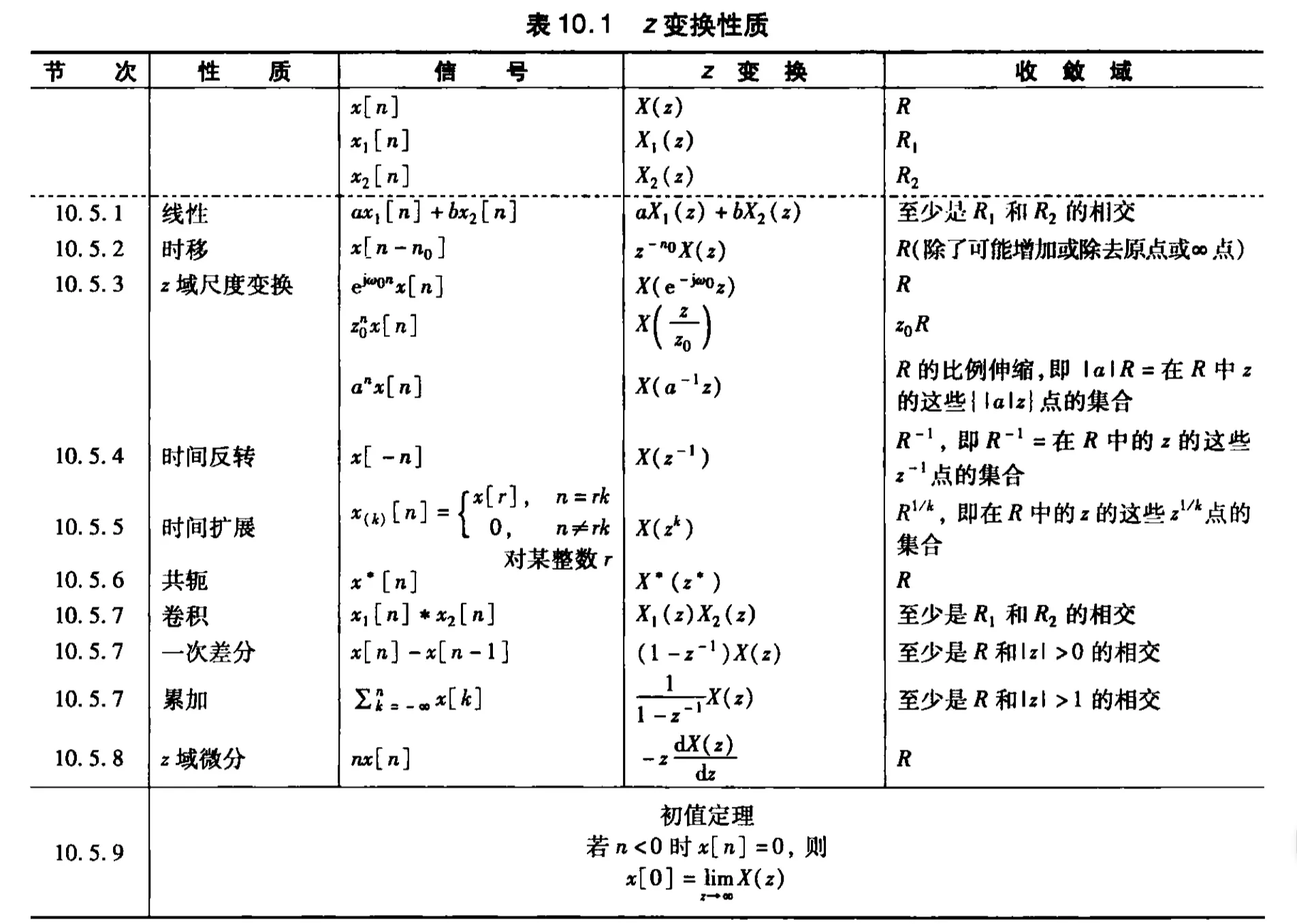
Properties of ZT
ZT pairs