[Lecture Notes] ShanghaiTech CS181 Artificial Intelligence

Lecture 1. Intro

Three types of approaches

1. Symbolism 符号

Representing knowledge with: symbols and their compositions (expressions). 用离散符号的组合表示knowledge.

Inference and learning: manipulating symbols.

Advantages: expressive; interpretable; rigorous. 表达能力强; 可解释,人可读; 有严密数理逻辑基础

Disadvantages: hard to learn; rigid. 难以学习; 脆弱.

2. Connectionism 连接主义

Representing knowledge with: interconnected networks of simple units (e.g. neural networks). 用大量简单计算单元的加权连接 (典型:神经网络)

Inference: follow the computation specified by the network.

Learning: optimization of connection weights.

Advantages: good performance; flexible. 表现好; 灵活

Disadvantages: black-box; data-hungry; hard to incorporate knowledge. 黑盒,人不可读,不可解释; 需大量训练数据; 难以融入先验知识

3. Statistical Approaches 基于统计的方法

Representing knowledge with: probabilistic models.

Inference and learning: probabilistic inference.

Advantages: interpretable; rigorous; learnable. 可解释; 严密; 可学习.

Disadvantages: less expressive; less flexible. 表达能力不如符号; 灵活性不如连接主义.

Course Overview

• Search
• Constraint satisfaction problems
• Game
• Propositional logic
• First-order predicate logic
• Probabilistic graphical models
• Probabilistic temporal models
• Probabilistic logics
• Markov decision processes
• Reinforcement learning
• Machine learning
• Introduction to natural language processing
• Introduction to computer vision

Lecture 2. Search

Search Problems

A Search problem consists of:

• A state space
• A successor function
• A start state and a goal test

World state: every detail of the environment

Search state: only the details needed for planning

$b$ is the branching factor (maximum number of child nodes).

$m$ is the max depth.

$s$ is the depth of the shallowest solution.

Num of nodes: $1 + b + b^2 + \cdots = O(b^m)$

Depth-First Search

Strategy: expand deepest node first.

Implementation: Fringe (a stack).

Time: $O(b^m)$ if $m$ is finite

Space: $O(bm)$ (because only has siblings on path to root)

Not complete (unless we prevent cycles).

Not optimal.

Breadth-First Search

Strategy: expand shallowest node first.

Implementation: fringe (a queue).

Time: $O(b^s)$.

Space: $O(b^s)$.

Complete.

Optimal only if all costs are $1$.

Iterative Deepening

Idea: get DFS’s space advantage with BFS’s time advantage.

Space: $O(bm)$

Time: $O(b^s)$

Complete and optimal (unit cost).

Uniform Cost Search

Strategy: expand cheapest node first.

Implementation: fringe (a priority queue, priority = cumulative cost).

Complete and optimal, but slow.

Greedy Search

Strategy: expand a node with smallest heuristic (estimate of distance to goal)

Fast, but not optimal, not complete.

A* search

Combine UCS with Greedy.

Optimal when heuristic is admissable (heuristic cost $\leq$ actual cost).

时空复杂度不会比UCS差.

• admissible: 估计的cost小于实际cost
• consistent: 相邻节点的heuristic之差小于这两个节点的距离

Tree search: admissible 则最优

Graph search (避免重复visit): consistent 则最优

Lecture 3. Constraint Satisfaction Problems 约束满足问题

Two types of search problems

• Planning = standard search problems
• Identification = constraint satisfaction problems (CSPs)

Backtracking Search 回溯搜索

Backtracking = DFS + variable-ordering + fail-on-violation

Filtering: Forward checking

Keep track of domains for unassigned variables and cross off bad options.

Filtering: constraint propagation

• Node consistency (1): Each node has valid value.

  任何一个节点有可选值

• Arc consistency (2): $X\to Y$ is consistent IFF for every $x$ in the tail there is some $y$ in the head which could be assigned without violating a constraint.

  $X\to Y$: 在X中随便选一个，Y仍然有得选

• K-consistency: For each $k$ nodes, any consistent assignment to $k-1$ can be extended to the $k^{th}$ node.

  对于任意$k$个点，不论$k-1$个点怎么选择，最后第$k$个点都有得选

• Strong k-consistency: also $k-1$, $k-2$, …, $1$-consistent.

Claim: Strong n-consistency means we can solve without backtracking.

Ordering: MRV (Min Remaining Value 最少剩余值)

Also called Most constrainted variable

Choose the variable with fewest legal left values in its domain

优先选择最少剩余量的选项 (选可选颜色数最少的点涂色)

Ordering: LCV (Least Constraining Value 最少约束值)

Choose the least constraining value (variable that rules out the fewest values in the remaining values)

优先排除掉可能让邻居可选值最少的值，给相邻变量的赋值留下最大的灵活性

Tree-structured CSPs

Theorem: If the constraint graph has no loops, the CSP can be solved in $O(nd^2)$ time.

Algorithm:

1. Order: parents precede children
2. Remove backward: for i in (n,2) removeInconsistent(Parent(Xi), i)
3. Assign forward: for i in (1,n) assign Xi consistently with Parent(Xi)

Nearly tree-structured CSPs

Cutset conditioning ?

Lecture 4. Adversarial search

Concepts

Value of a state: best achievable outcome (utility) from that state 能获得的最好成绩

Minimax value: best achievable utility against an optimal adversary 对手最优时可能获得的最好成绩

Minimax search

• Compute each nodes’s minimax value

• Implementation:

  

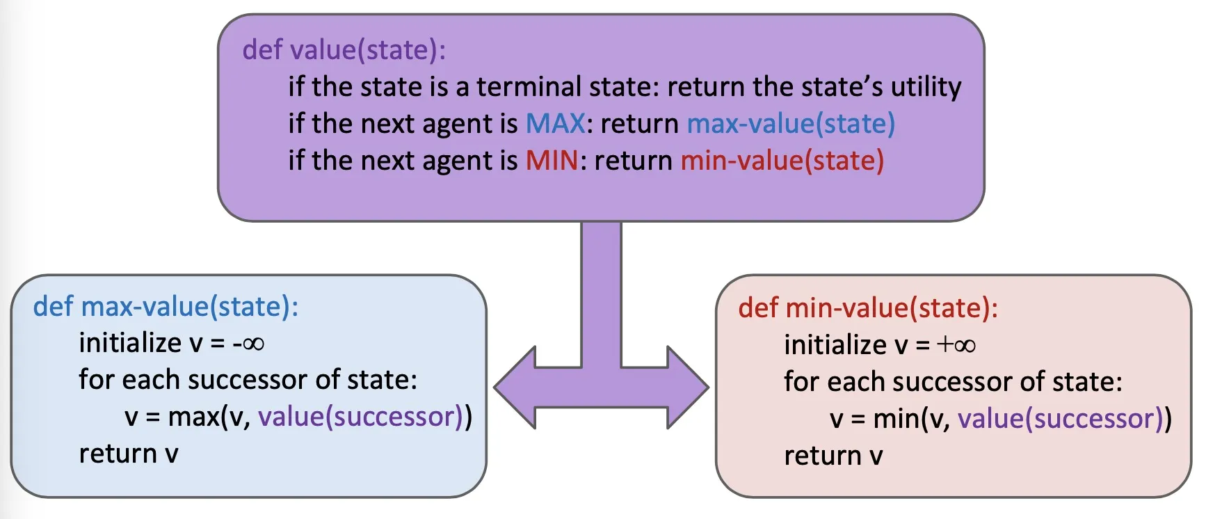
• Efficiency:

  Just like exhaustive DFS （相当于彻底的DFS搜索）

  Time: $O(b^m)$, Space: $O(bm)$

Depth-limited search (evalution functions)

• Search a limited depth.

• Replace terminal utilities with an evaluation function for non-terminal positions.

• Ideal evalution function: actual minimax value of the state

• Simple evalution function: weighted linear sum of features

• Idea: limit branching factor by considering only good moves

Alpha-Beta pruning

• Implementation

  

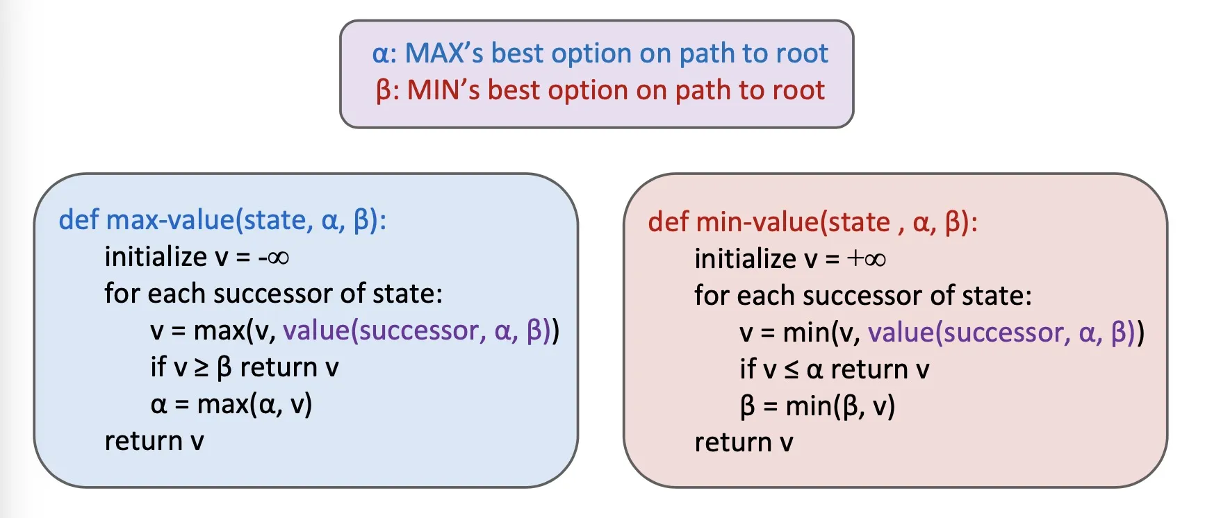
• $\alpha$-$\beta$ pruning 受到展开顺序的影响

Expectimax Search

• Compute average score under optimal play (expected utilities = weighted avg of children)

Mixed layer types

• Enviroment is an extra agent.
• E.g. You, a random ghost, and an optimal ghost

Multi-Agent Utilities

• Multiple players. Each player takes care of only his utility.

Lecture 5. Propositional Logic

Logic-based Symbolic AI

• Knowledge base

  contains sentences representing knowledge

  domain-specific

• Inference engine

  can answer questions by following the knowledge base

  domain-independent

Formal Language

Components of a formal language:

• Syntax: 语法
• Semantics: 语义 specifies the sentences is true/false in each model

PL (propositional logic)

• Negation: $\neg S$
• Conjunction: $S1 \land S2$ (and)
• Disjunction: $S1 \lor S2$ (or)
• Implication: $S1 \Rightarrow S2$
• Biconditional: $S1 \Leftrightarrow S2$

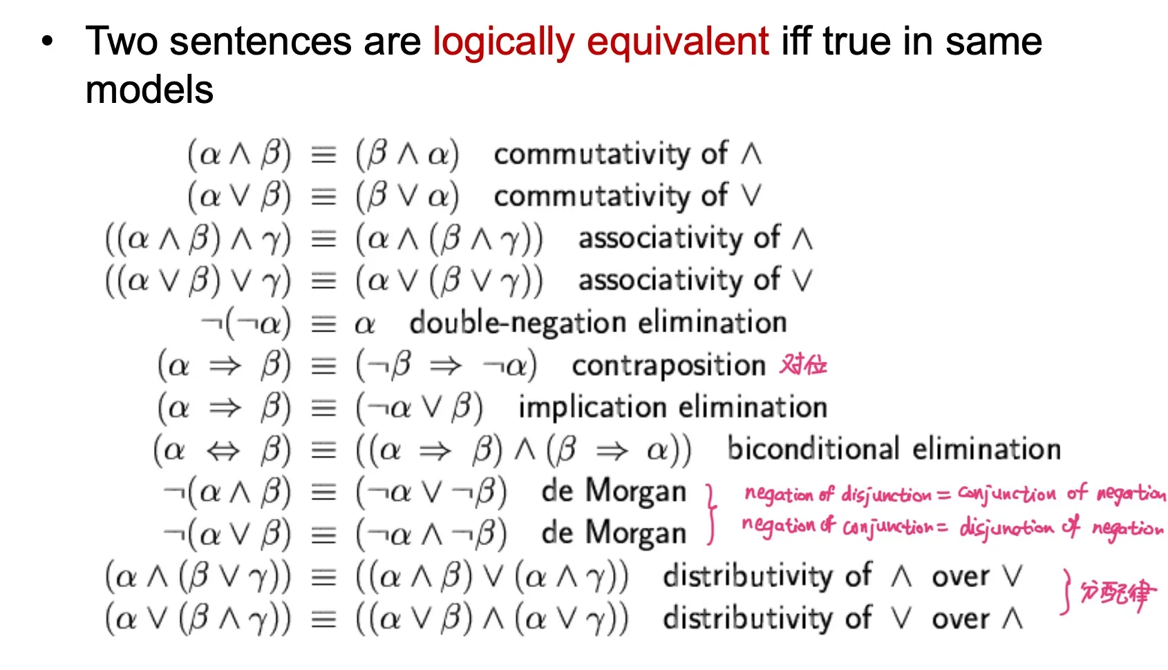
Logical equivalence

Validity and satisfiability

• valid: true in all models
• satisfiable: true in some models
• unsatisfiable: false in all models

Entailment

• $\alpha \vert= \beta$
• $models(\alpha) \subseteq models(\beta)$
• In every world where $\alpha$ is true, $\beta$ is also true.
• False entails everything.

Proof of entailment

A proof $A |= B$ is a demonstration of entailment from $A$ to $B$.

• Method 1: model checking 模型检验

  ​ 通过枚举所有可能得模型来检验。复杂度高。

• Method 2: application of inference rules

  • Search for a finite sequence of sentences each of which is an axiom or follows from preceding sentences by a rule of inference
    • axiom: 公理 a sentence known to be true
    • rule of inference: a function that takes one or more sentences (premises) and returns a sentence (conclusion)
  • Sound inference: 能证明出来的一定是entailed的
  • Complete inference: entailed的一定能被证明出来
  • 对于 Horn logic, Resolution 是 sound 和 complete 的

CNF (conjunctive normal form)

• conjunction of disjunctions of literals (clauses)

  • literal: a simple symbol or its negation: $A$ or $\neg A$
  • clause: disjunction of literals : $A\lor B$
  • CNF: conjunction of literals: $A \land B$

• conversion to CNF

  • 1: 把 $A\Leftrightarrow B$ 换成 $(A\Rightarrow B) \land (B\Rightarrow A)$
  • 2: 把 $A \Rightarrow B$ 换成 $\lnot A \lor B$
  • 3: 把 $\lnot (A\lor B)$换成 $\lnot A \land \lnot B$ ; $\lnot(A\land B)$ 换成 $\lnot A \lor \lnot B$
  • 4: 用分配律 ($\land$ over $\lor$)

Resolution

为了证明 $A|=B$, 我们去证明 $A \land \lnot B$ unsatisfiable.

• Step 1. Start from $A \land \lnot B$

• Step 2. Build a set $S$ of sub-formulas

  • Write $A \land \lnot B$ in CNF (写成 $P_1 \land P_2 \land \cdots \land P_k$ 形式)
  • Let $S = {P_1, \cdots, P_k}$

• Step 3. 对 $S$ 做 resolution: $(X\lor Y)\land (\lnot X \lor Z) \Rightarrow Y \lor Z$

  注: 不能说 $(X\lor Y)\land (\lnot X \lor Z) \equiv Y \lor Z$

• Reach an empty clause

Horn Logic

普通 propositional logic 的 Inference 通常NPC复杂.

Horn logic 用 forward / backward chaining 可实现线性复杂度.

• 形式: $P_1 \land P_2 \land \cdots \land P_n \Rightarrow Q$ 或 $\lnot P_1 \lor \lnot P_2 \lor \cdots \lor \lnot P_n \Rightarrow Q$

• Modus Ponens (MP规则): 所有前提fixed, 则结论 fixed

• Forward chaining: 从facts入手, 加入新fact直到得到query

• Backward chaining: 从query入手, 为证明query找前提条件

Forward chaining 对于 PL, FOL, Horn Logic 都是 sound 和 complete 的.

Backward chaining 对于 PL, FOL 是 sound 但 incomplete 的, 对于Horn是complete的.

Lecture 7. Bayesian Networks

• 概率

  条件概率: $P(a|b) = \frac{P(a, b)}{P(b)}$

  $p(y) p(x|y) = p(x,y)$

  Bayes rule: $p(x|y) = \frac{p(y|x) p(x)}{p(y)}$

  Chain rule: $p(a,b,c) = p(a) p(b|a) p(c|a,b)$

Syntax

贝叶斯网络语法:

• DAG (directed, acyclic graph) 有向无环图
• CPT (conditional probability table)
• CPT for each node given its parents (每个节点存有 给定父节点的条件概率分布)

Semantics

Global semantics

所有CPT相乘

Conditional independence semantics

给定父节点, 则该节点与非子孙节点独立

Independence 符号

$$X \perp\!\!\!\perp Y | Z$$

Markov blanket

Markov blanket consists of parents, children, children’s other parents (父,子,配偶)

Every variable is conditionally independent of all other variables given its Markov blanket.

给定markov blanket, 与所有其它变量条件独立

Common cause: 给定父节点(cause), 两个child(effects)独立

Common effect: 给定子节点(effect), 两个父节点(cause)不独立 (v-structure)

D-separation

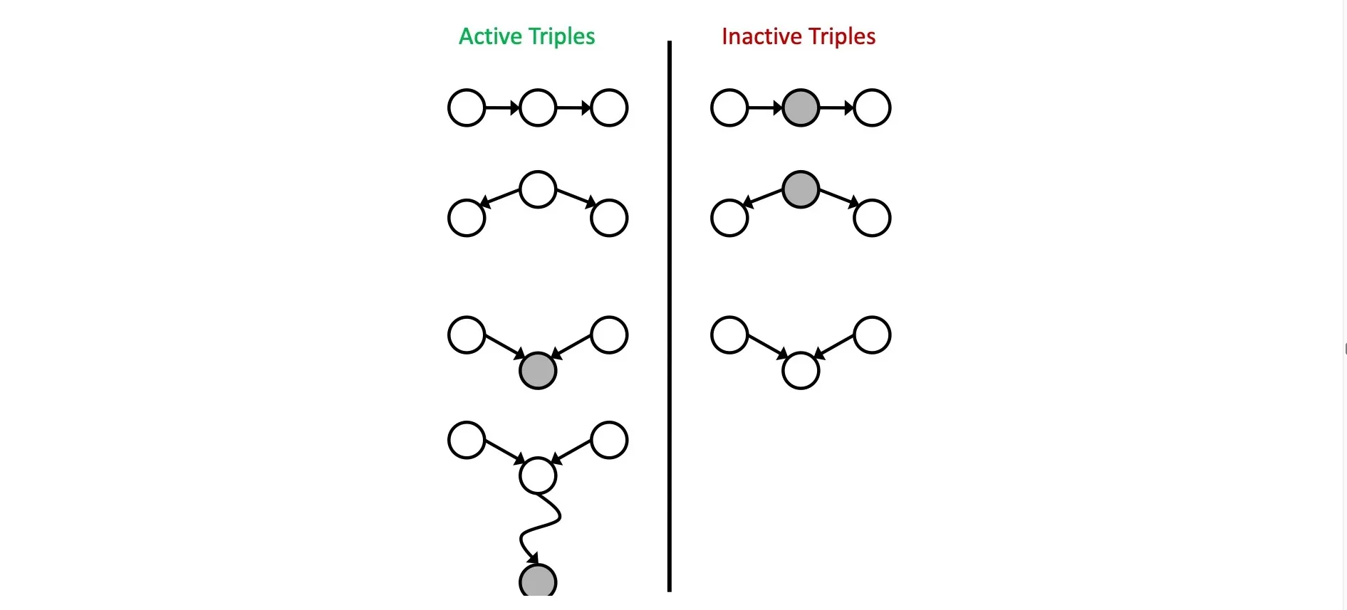
If all paths from X to Y are blocked (at least 1 inactive triple), then X is d-separated from Y by Z ($X \perp\!\!\!\perp Y | Z$)

Markov networks

undirected graph(无向图+clique全相连子图) + potentials 势函数(为每个clique的打分, 未经normalize, 不是概率)

• Undirected graph + potential functions

  • Undirected graph 无向图
  • For each clique or max clique, a potential function is defined

• 联合概率 正比于 势函数乘积

  $$p(x) = \frac{1}{Z} \prod_C \psi _C (\mathbf{x}_C)\\ Z = \sum_{\mathbf{x}} \prod_C \psi_C (\mathbf{x}_C)$$

  $\psi_C (\mathbf{x}_C)$ is the potential over clique $C$

  $Z$ is the normalization coefficient (partition function)

• Conditional Independence in Markov networks

  要判断$A\perp\!\!\!\perp B |C$, 只需判断从A到B的所有path是否都被C挡住了

• Markov blanket

  Markov blanket 就是这个节点的所有neighbor

Bayesian networks inference

Exact inference

Inference by enumeration

CPT相乘得联合概率, sum out 掉 hidden variables

• Evidence variables: $E_1, \cdots, E_k = e_1, \cdots, e_k$
• Query variable: $Q$ (我们想求: 给定$E$时$Q$的条件概率, 即 $P(Q|e_1, \cdots, e_k)$)
• Hidden variables: $H_1, \cdots, H_r$

Steps:

• Select the entries consistent with the evidence

• Sum out $H$ to get joint distribution of $Q$ and $E$

  $P(Q, e_1\cdots e_k) = \sum_{h1\cdots h_r} P(Q, h_1\cdots h_r, e_1\cdots e_k)$

• Normalize

  $Z = \sum_q P(Q, e_1,\cdots e_k)$

  $P(Q|e_1\cdots e_k) = \frac{1}{Z} P(Q, e_1\cdots e_k)$

Variable elimination

对每个 hidden variable 做 join and eliminate

指数复杂度, 但当贝叶斯网络为 poly tree 时, 为线性复杂度

Efficient inference on polytrees

Approximate Inference

Prior sampling

自顶向下采样

Rejection sampling

当采样与evidence不一致时丢弃

Likelihood weighting

只对non-evidence采样, 为每个样本计算weight (weight为所有evidence var条件概率的乘积)

$$\mathrm{weight} = \sum_{\mathrm{evidences}} p(\mathrm{evidence} | \mathrm{parent\ of\ evidence})$$

Gibbs sampling

顺序采样, 每个样本由之前样本修改而来, 得到序列

---

Lecture 12. Probabilistic temporal models

Markov models

(Assume discrete variables that share the same finite domain).

Values in the domain is called states.

The transition model $P(X_t|X_{t-1})$ specifies how the state evolves over time.

Stationarity assumption: same transition probabilities at all time steps.

Markov assumption: 给定$X_t$, $X_{t+1}, \cdots$ 与 $X_0, \cdots, X_{t-1}$ 条件独立

• 给定现在，过去与未来独立
• 每个时间点只与前一个有关
• First-order Markov Model

A k-th order model allows dependencies on $k$ earlier steps

Joint distribution: $P(X_0, \cdots, X_t) = P(X_0) \prod_t P(X_t | X_{t-1})$

Markov models 是不是 Bayes nets 的特例? Yes and No.

• Yes: 有向无环图, 联合概率 = 条件概率乘积
• No: 无限多变量, 重复的transition model 不符合 标准Bayes net syntax.

Forward algorithm

Given initial distribution $P(X_0)$

$$\begin{aligned} P(X_t) &= \sum_{x_{t-1}} P(X_t, X_{t-1} = x_{t-1})\\ &= \sum_{x_{t-1}} P(X_{t-1} = x_{t-1}) P(X_t|X_{t-1} = x_{t-1}) \end{aligned}$$

递归更新

对于大多数markov chain, 最初的分布带来的影响越来越小, converge到的 stationary distribution 与最初分布无关.

Stationary distribution: $P_\infty(X)$

$$P_{\infty}(X) = P_{\infty+1}(X) = \sum_x P(X|x) P_\infty (x)$$

Hidden markov models (HMM)

Only observe evidence $E$. Underlying markov chain over states $X$.

An HMM is defined by

• Initial distribution $P(X_0)$
• Transition model $P(X_t | X_{t-1})$
• Emission model $P(E_t | X_t)$

Joint distribution

$$P(X_0, \cdots, X_T, E_1, \cdots, E_T) = P(X_0) \prod_{t=1}^T P(X_t|X_{t-1})P(E_t|X_t)$$

Notation: $X_{a:b} = X_a, X_{a+1}, \cdots, X_b$

Filtering

给定所有evidence, 计算当前state的值的概率

Infer current state given all evidence: $P(X_t | e_{1:t})$

$$P(X_{t+1} | e_{1:t+1}) = \alpha \cdot P(e_{t+1}|X_{t+1})\cdot \sum_{x_t}P(X_t | e_{1:t})P(X_{t+1}|x_t)$$

May skip normalization $\alpha$.

每一步的复杂度是 $O(X^2)$, 其中 $X$ 是state数量

Most likely explanation

$\arg\max_{X_{0:t}} P(X_{0:t}|e_{1:t})$

The product of weights on a path is proportional to that state sequence’s probability.

Viterbi algorithm

For each state at time $t$, keep track of (unnormalized) maximum probability of any path to it.

$$m_{1:t+1} = \text{Viterbi}(m_{1:t}, e_{t+1}) = P(e_{t+1}|X_{t+1})\max_{x_t}P(X_{t+1}|x_t)m_{1:t}[x_t]$$

时间空间复杂度与 forward algorithm 相同.

Dynamic Bayes Nets (DBNs)

每个 HMM 都是 DBN.

每个 discrete DBN 都能用 HMM 表示.

每个 HMM state 都是 DBN state variables 的 Cartesian product.

Particle Filtering

Exact inference: variable elimination

Approximate inference by particle filtering

• Initially draw $N << |X|$ particles, each has weight 1
• Propagate forward: 根据 transition model 移动 particles
• Observe: 根据 emission model 给每个 particle 加上权重
• Resample: Draw N particles from the weighted sample distribution. 对加权后的sample重新采样, 采到的概率根据权重而定

如果没有 resample 这一步，那么 particle filtering 与 likelihood weighting 近似

---

Lecture 13. Markov decision processes

MDP

An MDP is defined by

• State $S$
• Actions $A$
• Transition function $T(s,a,s')$ or $P(s'|s,a)$
• Reward function $R(s,a,s')$ and discount $\gamma$
• Start state, terminal state

MDPs are non-deterministic search problems.

(In deterministic single-agent search problems, we want a plan, a sequence of actions)

For MDPs, we want an optimal policy $\pi^*: S \rightarrow A$

utility: sum of rewards

得到了MDP的policy之后，MDP表现得像关于policy的markov chain

Optimal quantities

• value / utility of a state $s$

  $V^*(s)$ is the expected utility starting in $s$ and acting optimally

• value / utility of a q-state $(s,a)$

  $Q^*(s,a)$ = expected utility starting out having taken action $a$ from state $s$ and thereafter acting optimally

Bellman equation

Value of states (recursive definition)

$$V^*(s) = \max_a Q^*(s,a)$$

$$Q^*(s,a) = \sum_{s'} T(s,a,s')\left[R(s,a,s') + \gamma V^*(s')\right]$$

Bellman equation

$$V^*(s) = \max_{a} \sum_{s'} T(s,a,s')\left[R(s,a,s') + \gamma V^*(s')\right]$$

Value iteration

Time limited values: $V_k(s)$ 是如果 $k$ 步之内结束, $s$ 的最佳值

Value iteration

• Starting with $V_0(s) = 0$

  $$V_{k+1}(s) = \max_a \sum_{s'} T(s,a,s')\left[R(s,a,s') + \gamma V_k^*(s')\right]$$

• Policy extraction (单步 expectimax)

  $$\pi^*(s) = \arg\max_a \sum_{s'} T(s,a,s')\left[R(s,a,s') + \gamma V^*(s')\right]$$

每一次迭代的复杂度: $O(S^2 A)$，$S$ 是state数量, $A$ 是action数量

Theorem: 一定会收敛到唯一的最佳值 converges to unique optimal.

Q-value iteration

• Starting with $Q_0(s, a) = 0$

  $$Q_{k+1}(s,a) = \sum_{s'} T(s,a,s')\left[R(s,a,s') + \gamma Q_k^*(s', a')\right]$$

• Policy extraction

  $$\pi^*(s) = \arg\max_a Q^*(s,a)$$

Policy iteration

Step 1: Policy evaluation

• Calculate utilities for some fixed (not optimal) policy

• Start with $V_0^\pi(s) = 0$

• Given $V_k^\pi$, calculate

  $$V_{k+1}^\pi(s) = \sum_{s'}T(s, \pi(s), s') \left[ R(s, \pi(s), s') + \gamma V_k^\pi(s') \right]$$

• Repeat until convergence

Step 2: Policy improvement

• Update policy using one-step look-ahead with resulting converged (not optimal) utilities as future values.

• One-step look-ahead

  $$\pi_{i+1}(s) = \arg \max_a \sum_{s'} T(s,a,s') \left[ R(s,a,s') + \gamma V^{\pi_i}(s') \right]$$

Repeat until policy converges.

policy iteration 第一步的复杂度是 $O(S^2)$ per iteration, 总复杂度是 $O(S^2A)$

Policy iteration is still optimal, can converge much faster under some conditions. (policy iteration 不一定比 value iteration 快 [2019 Fall Final])

---

Lecture 14. Reinforcement Learning

Model based learning

Learn an approximate model based on experiences.

Solve for values as if the learned model is correct.

Step 1. Learn empirical MDP model

• 对于每个 $s,a$ 记住(当前state, 采取action之后的结果 $s'$)
• Normalize 学习出 transition model $\hat{T}(s,a,s')$
• 遇到 $s,a,s'$ 时记下 reward $\hat{R}(s,a,s')$

Step 2. Solve the learned MDP

• e.g. Use value iteration

Passive reinforcement learning

给定固定的 policy $\pi(s)$, 但不知道 $T$, $R$.

Execute the policy and learn from experience to get state values.

Direct evaluation: 直接估计未来 reward 之和, 不记录 transition model

• 按照给定的 policy 去做
• 每次访问一个 state 时, 记下 sum of discounted rewards
• 取平均

Direct evaluation 好处:

• Easy to understand
• Does not require knowledge of $T$, $R$
• Can compute correct average values using just state transitions

缺点

• Wastes information about state connections
• Each state must be learned separately
• Take a long time to learn

Sample-based policy evaluation

$$V_{k+1}^\pi(s) = \sum_{s'} T(s, \pi(s), s') \left[R(s,\pi(s), s') + \gamma V_k^\pi(s')\right]$$

此处不知道T和R, 所以采用sample的方式

$$sample_1 = R(s,\pi(s), s_1') + \gamma V_k^\pi (s_1')\\ sample_n = R(s,\pi(s), s_n') + \gamma V_k^\pi (s_n')$$

$$V_{k+1}^\pi(s) = \frac{1}{n} \sum_i sample_i$$

Temporal Difference Learning

Idea: update $V(s)$ each time we experience a transition $(s,a,s',r)$

Sample of $V(s)$ is

$$sample = R(s, \pi(s), s') + \gamma V^\pi(s')$$

Update:

$$V^\pi(s) = (1-\alpha)V^\pi(s) + \alpha \cdot sample$$

(越新的sample越重要, forget about the past)

Q-learning

Sample-based Q-value iteration

$$Q_{k+1}(s,a) = \sum_{s'} T(s,a,s') \left[R(s,a,s') + \gamma \max_{a'}Q_k(s', a')\right]$$

Sample $(s,a,s',r)$ is

$$sample = R(s, \pi(s), s') + \gamma \max_{a'} Q(s', a')$$

Update new estimate

$$Q(s,a) = (1-\alpha) Q(s,a) + \alpha \cdot sample$$

Approximate Q-learning

当state太大的时候，用feature的加权求和代表state.

Approximate Q-learning 属于 model-free learning. [2019 Fall Final]

Reinforcement learning

​ MDP without knowing T and R

​ Offline planning VS online learning

Model based learning

Model free learning

​ Policy evaluation: Temporal Difference Learning

​ Exponential moving average

​ Computing q-values / policy: Q-learning

Exploration vs exploitation

​ random exploration, exploration function

Approximate Q-learning

​ Feature-based representation of states

---

Lecture 15. Supervised machine learning

Supervised learning

• Input: 有标注的训练集 $(x_j, y_j)$, $y_j = f(x_j)$
• Output: 尽可能接近 target function $f$ 的函数 $h$ (hypothesis)

Supervised learning 的类型

• Classification: 离散输出
• Regression: real-valued 输出
• Structured: structured 输出

Naive bayes classifer

Naive bayes model:

$$P(Y, F_1, \cdots, F_n) = P(Y) \prod_i P(F_i|Y)$$

所做的假设: 给定label $Y$, 所有features独立

总参数与$n$呈线性关系

Bag-of-words naive bayes

Features: $W_i$ is the word at position $i$

$$P(Y, W_1, \cdots, W_n) = P(Y) \prod_i P(W_i|Y)$$

Each word is identically distributed.

All positions share the same conditional probabilities $P(W|Y)$. 所有位置CPT相同

Called ‘bag-of-words’ because model is insensitive to word order or reordering.

Inference for naive bayes

Goal: $P(Y|f_1, \cdots, f_n)$

Step1. Get joint probability of label and evidence for each label

将所有CPT相乘

Step2. Normalization

Maximum likelihood estimation

empirical rate (frequency of seeing this outcome)

$$P_{ML}(x) = \frac{\mathrm{count}(x)}{\mathrm{total\ samples}}$$

Using empirical rate will overfit the training data.

Important concepts

Learn parameters (e.g. model probabilities) on training set

Tune hyperparameters on held-out set

Compute accuracy of test set

Overfitting: learn to fit the training data very closely, but fit the test data poorly

Generalization: try to fit the test data as well

过拟合产生的原因

• 训练集不能代表真实的数据分布
  • 训练集太少 或 训练集噪声太多
• 太多attributes, 部分属性与分类任务无关
• 模型过于 expressive

避免overfitting

• 更多训练集
• 去除无关属性
• 使用正则化、提前停止、pruning等手段限制模型的expressiveness

Laplace smoothing

Laplace’s estimate: pretend you saw every outcome k extra times

$$P_{LAP}(x) = \frac{c(x)+k}{\sum_x \left[c(x)+k\right]}$$

Linear classifiers (perceptrons)

Inputs are feature values. Each feature has a weight.

Sum is the activation.

Output +1 if $w\cdot f(x) +b > 0$, -1 otherwise

训练(更新): $w=w+y^*\cdot f$

---

Lecture 16. Unsupervised machine learning

Clustering

K-means

Voronoi diagram: partitions the space by nearest cluster center

Consider the total distance to the means

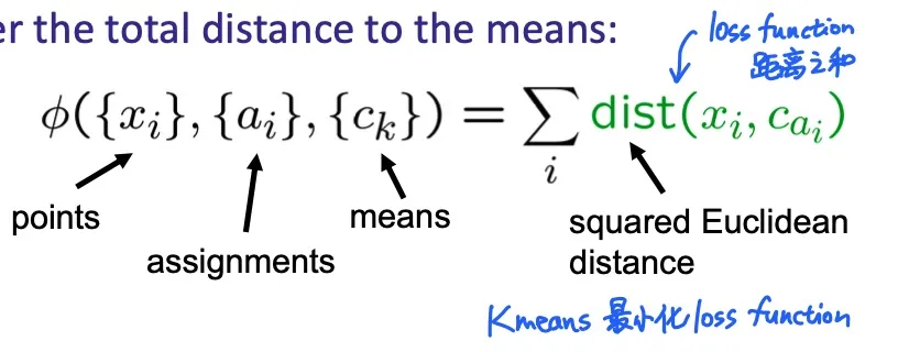
Two stages

• fix means c, update assignments a
• fix assignments a, update means c

EM

EM can be used to learn any model with hidden variables (missing data). [Fall 2019 Final]

• E-step: Assign data instances proportionately to different models 计算每个数据点属于不同cluster的可能性分布

  $$P(y_j = i | x_j, \theta^{(t)}) \propto \pi_i^{(t)} N(x_j | \mu_i^{(t)}, {\Sigma}_i ^{(t)})$$

• M-step: Revise each cluster model based on its proportionately assigned points. 更新cluster的分布

GMM (Gaussian mixture model / mixture of Gaussians)

当使用EM学习GMM时, M-step计算的是weighted maximum likelihood estimation (MLE).

当 all the Gaussians are spherical and have identical weights and covariances, with hard assignments 的时候, EM降级成k-means

---

Lecture 16. NLP 自然语言处理

Constituency Parsing

Constituent parse tree (phrase structure)

每个中间的节点代表一个 phrase / constituent

Grammar: the set of constituents and the rules that govern how they combine

Context-free grammars (CFGs) (phrase structure grammars) 四个组成部分

• A set $\Sigma$ of terminals (words)
• A set $N$ of nonterminals (phrases)
• A start symbol $S\in N$
• A set $R$ of production rules (specifies how a nonterminal can produce a string of terminals and/or nonterminals)

Dependency grammar: focus on binary relations among words. (CFG focus on constituents)

Sentence generation

• 使用grammar生成string
• 从仅有 start symbol $S$ 开始, 递归地使用rules重写句子直到只剩下 terminals

Sentence Parsing

• Taking a string and grammar, return one or more parse trees for that string
• Probabilistic grammars (stochastic grammars): 每条规则具有概率, parse tree的概率是使用过的每条规则的概率之积
• Ambiguity: 如果一句话有两个或以上的可能得parse tree, 则 ambiguous

Parsing algorithm

A brute-force approach

• Enumerate all parse trees consistent with the input string
• Problem: # of binary trees with $n$ leaves is $C_{n-1}$ (exponential growth)

CYK algorithm

• A bottom-up dynamic programming algorithm

• Applies to CFG in Chomsky Normal Form (CNF)

  • 仅两种production rules: A → BC 和 A → w
  • 任何CFG都能转化为CNF
  • Probabilistic CFGs tend to assign larger probabilities to smaller parse trees. [Fall 2019 Final]

• Build a table so that a non-terminal A spanning from i to j is placed in [i-1, j]

• S (span整个string) 应该位于 [0, n]

• Base case: 如果有一条规则 $A\to w_i$，则 $A$ 应该在 [i-1, i] 的位置

• Recursion: 如果 $A \to B C$, $B$ 在 [i,k], $C$ 在 [k, j], 则 $A$ 在 [i, j]

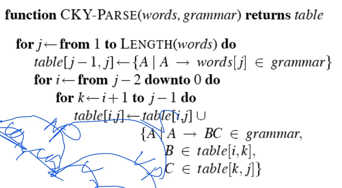
• Probabilistic parsing: 在运行CYK算法的时候，在 [i-1, j] 时，对于每个中间节点A添上最可能的由A出发覆盖 [i,j] substring 的parse tree的概率

Dependency Parsing

• A dependency parse is a directed tree where
  • nodes are the words in a sentence (ROOT 是一个特殊的根节点)
  • links between words represent their dependency relations

Lecture 18. Final Review

That’s all!